Skip to content

Advanced

Writing a custom mapper

OrdBoostRegressor accepts any custom mapper that inherits from BaseBinMapper. In this example, we will show how to create a new mapper. A minimal mapper only needs to implement the _intra_bin_points method that defines which points to add between the bin edges and their associated weight.

Below is the simplest mapper to implement: the NullBinMapper. It does not add any points to the grid. Therefore, the CDFs will only be evaluated at the bin edges.

NOTE: This mapper is equivalent to using the UniformBinMapper with n_points=0.

class NullBinMapper(BaseBinMapper):
    """Maps discrete bin probabilities using raw bin edges only, with no
    intra-bin refinement.

    This is the minimal possible BaseBinMapper subclass: _intra_bin_points
    returns no interior points, so the fitted CDF is a straight
    piecewise-linear interpolation directly across bin_edges (equivalent
    to assuming uniform probability density within each bin). This is
    functionally identical to UniformBinMapper(n_points=0) -- the package
    already ships this exact null mapper -- and is included here purely
    to show the minimal _intra_bin_points implementation a custom mapper
    can have. See :doc:`../concepts` for why a null mapper is a useful
    baseline when evaluating whether a more elaborate mapper is actually
    adding value.
    """

    def _intra_bin_points(self, bin_data: np.ndarray, low: float, high: float, k: int):
        """Return no interior points -- boundary points from
        BaseBinMapper._build_grid alone define the grid.

        Parameters
        ----------
        bin_data : ndarray of shape (n_bin_samples,)
            Continuous training targets belonging to bin `k`. Unused
        low : float
            The effective lower boundary of bin `k`. Unused
        high : float
            The effective upper boundary of bin `k`. Unused
        k : int
            The 0-indexed bin number. Unused

        Returns
        -------
        points : ndarray of shape (1,)
            An empty array of points that are added to the grid.
        weights : ndarray of shape (1,)
            An empty of weights that are added to the grid CDF weights.

        """
        return np.array([]), np.array([])

Once the new mapper has been defined, we can now use it when creating an OrdBoostRegressor:

# Plug the custom mapper into OrdBoostRegressor

# Generate some synthetic data
rng = np.random.default_rng(42)
n_samples = 500
X = rng.standard_normal((n_samples, 3))
# Positive, right-skewed target (e.g. a duration or cost outcome)
y = np.exp(1.0 + 0.5 * X[:, 0] + rng.standard_normal(n_samples) * 0.3)

# Pass an *unconfigured* mapper instance (no bin_edges set)
# OrdBoostRegressor is the single source of truth for bin_edges
# and assigns them automatically.
custom_mapper = NullBinMapper()

model = OrdBoostRegressor(n_bins=8, mapper=custom_mapper, random_state=42)
model.fit(X, y)

n = 5  # Get the n first CDFs
dist = model.predict_dist(X[:n])
medians = dist.median()
pis = dist.interval(alpha=0.05)  # 95% prediction interval
for i in range(n):
    print(f"Sample {i} median [95% PI]")
    print(f"  {medians[i]:.2f} [{pis[0][i]:.2f} -- {pis[1][i]:.2f}]")

Running this example should produce the following output:

Sample 0 median [95% PI]
  2.76 [1.50 -- 3.10]
Sample 1 median [95% PI]
  3.60 [3.12 -- 6.76]
Sample 2 median [95% PI]
  4.44 [1.78 -- 5.15]
Sample 3 median [95% PI]
  1.96 [1.41 -- 2.49]
Sample 4 median [95% PI]
  2.98 [2.24 -- 3.92]

Full example:

Writing a custom mapper
import numpy as np

from ordboost.mappers import BaseBinMapper
from ordboost.models import OrdBoostRegressor


# --- Mapper definition
class NullBinMapper(BaseBinMapper):
    """Maps discrete bin probabilities using raw bin edges only, with no
    intra-bin refinement.

    This is the minimal possible BaseBinMapper subclass: _intra_bin_points
    returns no interior points, so the fitted CDF is a straight
    piecewise-linear interpolation directly across bin_edges (equivalent
    to assuming uniform probability density within each bin). This is
    functionally identical to UniformBinMapper(n_points=0) -- the package
    already ships this exact null mapper -- and is included here purely
    to show the minimal _intra_bin_points implementation a custom mapper
    can have. See :doc:`../concepts` for why a null mapper is a useful
    baseline when evaluating whether a more elaborate mapper is actually
    adding value.
    """

    def _intra_bin_points(self, bin_data: np.ndarray, low: float, high: float, k: int):
        """Return no interior points -- boundary points from
        BaseBinMapper._build_grid alone define the grid.

        Parameters
        ----------
        bin_data : ndarray of shape (n_bin_samples,)
            Continuous training targets belonging to bin `k`. Unused
        low : float
            The effective lower boundary of bin `k`. Unused
        high : float
            The effective upper boundary of bin `k`. Unused
        k : int
            The 0-indexed bin number. Unused

        Returns
        -------
        points : ndarray of shape (1,)
            An empty array of points that are added to the grid.
        weights : ndarray of shape (1,)
            An empty of weights that are added to the grid CDF weights.

        """
        return np.array([]), np.array([])


# --- Usage
# Plug the custom mapper into OrdBoostRegressor

# Generate some synthetic data
rng = np.random.default_rng(42)
n_samples = 500
X = rng.standard_normal((n_samples, 3))
# Positive, right-skewed target (e.g. a duration or cost outcome)
y = np.exp(1.0 + 0.5 * X[:, 0] + rng.standard_normal(n_samples) * 0.3)

# Pass an *unconfigured* mapper instance (no bin_edges set)
# OrdBoostRegressor is the single source of truth for bin_edges
# and assigns them automatically.
custom_mapper = NullBinMapper()

model = OrdBoostRegressor(n_bins=8, mapper=custom_mapper, random_state=42)
model.fit(X, y)

n = 5  # Get the n first CDFs
dist = model.predict_dist(X[:n])
medians = dist.median()
pis = dist.interval(alpha=0.05)  # 95% prediction interval
for i in range(n):
    print(f"Sample {i} median [95% PI]")
    print(f"  {medians[i]:.2f} [{pis[0][i]:.2f} -- {pis[1][i]:.2f}]")

Bounded data and atoms

This example demonstrates the use of the lower_bound and upper_bound attributes with and whitout atoms. We will look at the effects these have on the model. Let's start by generating some synthetic data. For this example, we want to include a floor atom at y=0 (zero-inflation) and a ceiling bound at y=10 with no atom. This means that the target values y can be 0, and they approach 10 without reaching. We are creating 10,000 samples with 8 features. We then modify the target so that it is bound between 0 and 10, and zero-inflated (roughly 50% of data at 0).

import matplotlib.pyplot as plt
import numpy as np
from sklearn.datasets import make_regression
from sklearn.metrics import mean_absolute_error
from sklearn.model_selection import train_test_split

from ordboost import OrdBoostRegressor
from ordboost.metrics import (
    baseline_distribution,
    crps_score,
    crps_skill_score,
    interval_coverage_rate,
    marginal_calibration_curve,
    pit_diagnostics,
    sharpness,
    winkler_score,
)

# --- Generate data
rng = np.random.default_rng(42)
n_samples = 10000
upper_bound = 10.0

regression_data = make_regression(
    n_samples=n_samples,
    n_features=8,
    n_informative=4,
    noise=3.0,
    random_state=42,
)
X = regression_data[0]
latent = regression_data[1]

latent_std = (latent - latent.mean()) / latent.std()  # rescale to a controlled range

# Zero-inflation: a clean, sharp logistic in the single latent driver
# (easy for the classifier to recover).
zero_prob = 1.0 / (1.0 + np.exp(-3.0 * latent_std))
is_zero = rng.random(n_samples) < zero_prob

# Continuous part: Beta parameterized by (mean, concentration) rather than
# a raw shape parameter.
beta_mean = 0.3 + 0.5 * (latent_std - latent_std.min()) / (
    latent_std.max() - latent_std.min()
)
beta_mean = np.clip(beta_mean, 0.05, 0.95)
concentration = 9.0
a = beta_mean * concentration
b = (1.0 - beta_mean) * concentration
continuous_part = upper_bound * rng.beta(a, b, size=n_samples)

y = np.where(is_zero, 0.0, continuous_part)
X_train, X_test, y_train, y_test = train_test_split(X, y, random_state=42)

# Plot y_test
fig, ax = plt.subplots(figsize=(7, 5))
ax.hist(y_test, bins=20, edgecolor="black")
ax.set_xlabel("Target")
ax.set_ylabel("Density (log)")
ax.set_yscale("log")
ax.set_title("Prediction target on a log scale")
plt.show()

The code should generate the following figure showing the target test distribution:
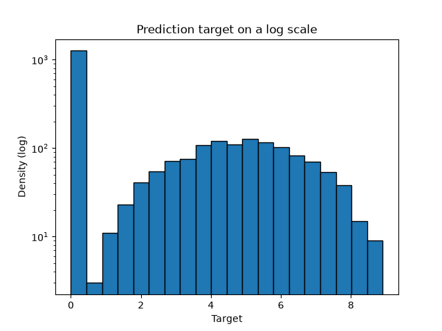
y_test distribution

NOTE: the target has a large amount of data at 0 and never reaches 10.

Now that the data has been generated, we can fit our models. First, we define some bin edges that cover the 0 to 10 range. We then create two models, one with the mapper_kwargs and one without. The models have identical hyperparameters and use the quantile bin mapper. The first model defines four mapper_kwargs, the lower_bound and upper_bound values are floats corresponding to the limits we have imposed on the data. The floor_atom is set to True because there is data at 0, however, the ceiling_atom is set to False because y never reaches 10.

Once the models have been created, we can fit them with the train data and generate the predictions and distributions.

bin_edges = [1.0, 2.5, 5.0, 7.5, 9.0]

model = OrdBoostRegressor(
    mapper="quantile",
    bin_edges=bin_edges,
    monotonicity="isotonic",
    max_iter=200,
    learning_rate=0.01,
    random_state=42,
    mapper_kwargs={
        "lower_bound": 0.0,
        "floor_atom": True,
        "upper_bound": upper_bound,
        "ceiling_atom": False,
    },
)

model_no_bounds = OrdBoostRegressor(
    mapper="quantile",
    bin_edges=bin_edges,
    monotonicity="isotonic",
    max_iter=200,
    learning_rate=0.01,
    random_state=42,
)

# Fit and predict with the bounded model
model.fit(X_train, y_train)
y_pred = model.predict(X_test)
dist_test = model.predict_dist(X_test)

# Fit and predict with the boundless model
model_no_bounds.fit(X_train, y_train)
y_pred_no_bounds = model_no_bounds.predict(X_test)
dist_test_no_bounds = model_no_bounds.predict_dist(X_test)

Now let us evaluate the model to see the effects of the bounds and atoms. First, let us look at the accuracy and skill scores with the MAE, CRPS, and CRPSS for both models.

mae = mean_absolute_error(y_test, y_pred)
crps = crps_score(y_test, dist_test)

dist_baseline = baseline_distribution(y_train, n_samples=len(y_test))
crpss = crps_skill_score(y_test, dist_test, dist_baseline)

mae_no_bounds = mean_absolute_error(y_test, y_pred_no_bounds)
crps_no_bounds = crps_score(y_test, dist_test_no_bounds)
crpss_no_bounds = crps_skill_score(y_test, dist_test_no_bounds, dist_baseline)

print("        Bounded | Boundless")
print(f"MAE:     {mae:.3f}  |    {mae_no_bounds:.3f}")
print(f"CRPS:    {crps:.3f}  |    {crps_no_bounds:.3f}")
print(f"CRPSS:   {crpss:.3f}  |    {crpss_no_bounds:.3f}")

The code will generate the following table:

        Bounded | Boundless
MAE:     1.712  |    1.745
CRPS:    0.993  |    1.005
CRPSS:   0.313  |    0.305

Both model exhibit similar performances, with the bounded model showing a marginal improvement over the boundless model (lower CRPS and MAE and higher CPRSS). Now let us take a look at the prediction intervals. We compute the interval coverage rate, the sharpness, and the Winkler score at difference significance levels and plot the results.

coverage_levels = np.arange(10, 91, 10)  # nominal coverage in percent
alphas = 1.0 - coverage_levels / 100.0

empirical_coverage = np.array(
    [
        interval_coverage_rate(
            y_test, dist_test, alpha=a, tolerance=model.mapper_.boundary_epsilon
        )
        for a in alphas
    ]
)
interval_sharpness = np.array([sharpness(dist_test, alpha=a) for a in alphas])
winkler = np.array([winkler_score(y_test, dist_test, alpha=a) for a in alphas])

empirical_coverage_no_bounds = np.array(
    [interval_coverage_rate(y_test, dist_test_no_bounds, alpha=a) for a in alphas]
)
interval_sharpness_no_bounds = np.array(
    [sharpness(dist_test_no_bounds, alpha=a) for a in alphas]
)
winkler_no_bounds = np.array(
    [winkler_score(y_test, dist_test_no_bounds, alpha=a) for a in alphas]
)

fig, axes = plt.subplots(1, 3, figsize=(15, 4))

axes[0].plot(
    coverage_levels,
    empirical_coverage * 100,
    color="b",
    marker="o",
    label="Bounded",
)
axes[0].plot(
    coverage_levels,
    empirical_coverage_no_bounds * 100,
    color="r",
    marker="s",
    label="Boundless",
)
axes[0].plot([0, 100], [0, 100], linestyle="--", color="black")
axes[0].legend()
axes[0].set_xlabel("Nominal coverage (%)")
axes[0].set_ylabel("Empirical coverage (%)")
axes[0].set_title("Coverage reliability")

axes[1].plot(
    coverage_levels, interval_sharpness, color="b", marker="o", label="Bounded"
)
axes[1].plot(
    coverage_levels,
    interval_sharpness_no_bounds,
    color="r",
    marker="s",
    label="Boundless",
)
axes[1].legend()
axes[1].set_xlabel("Nominal coverage (%)")
axes[1].set_ylabel("Mean interval width")
axes[1].set_title("Sharpness")

axes[2].plot(coverage_levels, winkler, marker="o", color="b", label="Bounded")
axes[2].plot(
    coverage_levels,
    winkler_no_bounds,
    color="r",
    marker="s",
    label="Boundless",
)
axes[2].legend()
axes[2].set_xlabel("Nominal coverage (%)")
axes[2].set_ylabel("Winkler score")
axes[2].set_title("Winkler score")

fig.tight_layout()
plt.show()

The code will generate the following results:
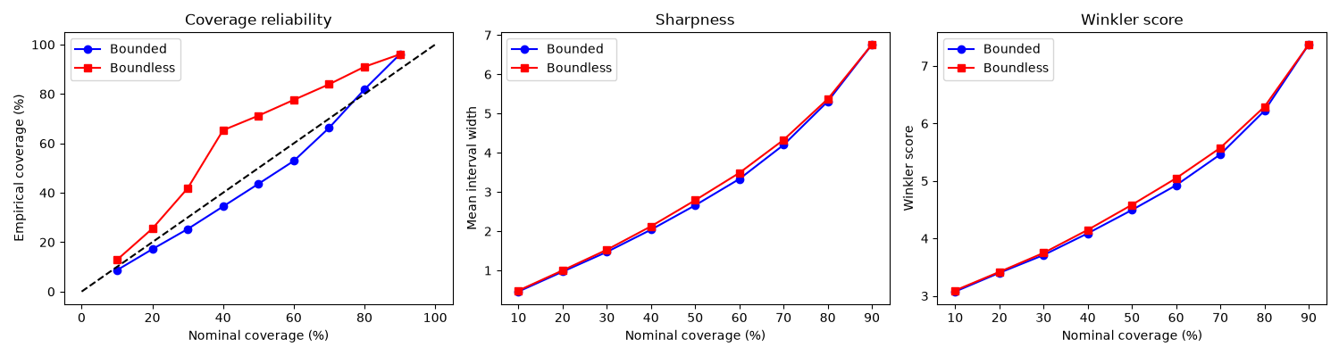
prediction_intervals

Now the difference between the bounded and boundless model becomes more apparent. The boundless model has too much coverage, the true value falls in the interval more often then expected. On the other hand, the bounded model has too little coverage. Both model have similar sharpness and Winkler scores.

Finally, let's look at the calibration. We will compute the PIT histograms and the marginal calibration curves for both models and plot the results.

# Marginal calibration: aggregate comparison of the empirical CDF against
# the average predicted CDF across all test samples.
grid_y, calibration = marginal_calibration_curve(y_test, dist_test, model.mapper_)
grid_y_no_bounds, calibration_no_bounds = marginal_calibration_curve(
    y_test, dist_test_no_bounds, model_no_bounds.mapper_
)

fig, ax = plt.subplots(figsize=(7, 5))
ax.plot(grid_y, calibration, color="b", linewidth=2, label="Bounded")
ax.plot(
    grid_y_no_bounds,
    calibration_no_bounds,
    color="r",
    linewidth=2,
    label="Boundless",
)
ax.axhline(0.0, color="black", linestyle="--", linewidth=1)
ax.legend()
ax.set_xlabel("y")
ax.set_ylabel(r"eCDF $-\ \overline{CDF}$")
ax.set_title("Marginal calibration curve")
plt.show()

# Randomized PIT histogram: per-sample calibration check, aware of the
# floor atom via model.mapper_.floor_atom (True here) and correctly
# treating the ceiling as a plain boundary rather than an atom, since
# model.mapper_.ceiling_atom is False.
pit = pit_diagnostics(y_test, dist_test, model.mapper_, resolution=1e-6)
hist = pit.hist_values(bins=20)
alpha_score = pit.alpha_score()

pit_no_bounds = pit_diagnostics(
    y_test,
    dist_test_no_bounds,
    model_no_bounds.mapper_,
    resolution=1e-6,
)
hist_no_bounds = pit_no_bounds.hist_values(bins=20)
alpha_score_no_bounds = pit_no_bounds.alpha_score()
fig, ax = plt.subplots(figsize=(7, 5))
ax.bar(
    hist["bin_centre"].values - 0.3 / 20,
    np.asarray(hist.values),
    width=0.3 / 20,
    color="b",
    edgecolor="black",
    label=rf"Bounded ($\alpha$ score = {alpha_score:.3f})",
)
ax.bar(
    hist_no_bounds["bin_centre"].values + 0.1 / 20,
    np.asarray(hist_no_bounds.values),
    width=0.3 / 20,
    color="r",
    edgecolor="black",
    label=rf"Boundless ($\alpha$ score = {alpha_score_no_bounds:.3f})",
)
ax.axhline(1.0 / 20, color="black", linestyle="--", linewidth=1, label="Uniform")
ax.set_xlabel("PIT value")
ax.set_ylabel("Proportion")
ax.set_title("PIT histograms")
ax.legend()
plt.show()

The code will generate the following results:
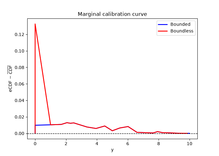
marginal_calibration

The marginal calibration clearly shows a difference between the bounded and the boundless model near 0. This is exactly where the floor atom is located. Without the floor atom and lower bound set, the model is miscalibrated in that lower region. The upper bound also shows an effect however much weaker than at the floor.
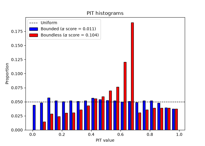
PIT

The PIT histograms corroborate the results from the marginal calibration. The boundless model systematically underestimates the target values which creates a PIT histogram with a peak near 0.6 and \(\alpha\) score of 0.104. In contrast, the bounded model has PIT histogram that is near uniform and an \(\alpha\) score of 0.011, 10 times smaller.

These results clearly show the effects of using the atoms and bounds to constrain the models.

Full example:

Bounds and atoms
import matplotlib.pyplot as plt
import numpy as np
from sklearn.datasets import make_regression
from sklearn.metrics import mean_absolute_error
from sklearn.model_selection import train_test_split

from ordboost import OrdBoostRegressor
from ordboost.metrics import (
    baseline_distribution,
    crps_score,
    crps_skill_score,
    interval_coverage_rate,
    marginal_calibration_curve,
    pit_diagnostics,
    sharpness,
    winkler_score,
)

# --- Generate data
rng = np.random.default_rng(42)
n_samples = 10000
upper_bound = 10.0

regression_data = make_regression(
    n_samples=n_samples,
    n_features=8,
    n_informative=4,
    noise=3.0,
    random_state=42,
)
X = regression_data[0]
latent = regression_data[1]

latent_std = (latent - latent.mean()) / latent.std()  # rescale to a controlled range

# Zero-inflation: a clean, sharp logistic in the single latent driver
# (easy for the classifier to recover).
zero_prob = 1.0 / (1.0 + np.exp(-3.0 * latent_std))
is_zero = rng.random(n_samples) < zero_prob

# Continuous part: Beta parameterized by (mean, concentration) rather than
# a raw shape parameter.
beta_mean = 0.3 + 0.5 * (latent_std - latent_std.min()) / (
    latent_std.max() - latent_std.min()
)
beta_mean = np.clip(beta_mean, 0.05, 0.95)
concentration = 9.0
a = beta_mean * concentration
b = (1.0 - beta_mean) * concentration
continuous_part = upper_bound * rng.beta(a, b, size=n_samples)

y = np.where(is_zero, 0.0, continuous_part)
X_train, X_test, y_train, y_test = train_test_split(X, y, random_state=42)

# Plot y_test
fig, ax = plt.subplots(figsize=(7, 5))
ax.hist(y_test, bins=20, edgecolor="black")
ax.set_xlabel("Target")
ax.set_ylabel("Density (log)")
ax.set_yscale("log")
ax.set_title("Prediction target on a log scale")
plt.show()

# --- Create and fit models
bin_edges = [1.0, 2.5, 5.0, 7.5, 9.0]

model = OrdBoostRegressor(
    mapper="quantile",
    bin_edges=bin_edges,
    monotonicity="isotonic",
    max_iter=200,
    learning_rate=0.01,
    random_state=42,
    mapper_kwargs={
        "lower_bound": 0.0,
        "floor_atom": True,
        "upper_bound": upper_bound,
        "ceiling_atom": False,
    },
)

model_no_bounds = OrdBoostRegressor(
    mapper="quantile",
    bin_edges=bin_edges,
    monotonicity="isotonic",
    max_iter=200,
    learning_rate=0.01,
    random_state=42,
)

# Fit and predict with the bounded model
model.fit(X_train, y_train)
y_pred = model.predict(X_test)
dist_test = model.predict_dist(X_test)

# Fit and predict with the boundless model
model_no_bounds.fit(X_train, y_train)
y_pred_no_bounds = model_no_bounds.predict(X_test)
dist_test_no_bounds = model_no_bounds.predict_dist(X_test)

# --- CRPS and skill score

mae = mean_absolute_error(y_test, y_pred)
crps = crps_score(y_test, dist_test)

dist_baseline = baseline_distribution(y_train, n_samples=len(y_test))
crpss = crps_skill_score(y_test, dist_test, dist_baseline)

mae_no_bounds = mean_absolute_error(y_test, y_pred_no_bounds)
crps_no_bounds = crps_score(y_test, dist_test_no_bounds)
crpss_no_bounds = crps_skill_score(y_test, dist_test_no_bounds, dist_baseline)

print("        Bounded | Boundless")
print(f"MAE:     {mae:.3f}  |    {mae_no_bounds:.3f}")
print(f"CRPS:    {crps:.3f}  |    {crps_no_bounds:.3f}")
print(f"CRPSS:   {crpss:.3f}  |    {crpss_no_bounds:.3f}")

# --- Prediction interval evaluation

coverage_levels = np.arange(10, 91, 10)  # nominal coverage in percent
alphas = 1.0 - coverage_levels / 100.0

empirical_coverage = np.array(
    [
        interval_coverage_rate(
            y_test, dist_test, alpha=a, tolerance=model.mapper_.boundary_epsilon
        )
        for a in alphas
    ]
)
interval_sharpness = np.array([sharpness(dist_test, alpha=a) for a in alphas])
winkler = np.array([winkler_score(y_test, dist_test, alpha=a) for a in alphas])

empirical_coverage_no_bounds = np.array(
    [interval_coverage_rate(y_test, dist_test_no_bounds, alpha=a) for a in alphas]
)
interval_sharpness_no_bounds = np.array(
    [sharpness(dist_test_no_bounds, alpha=a) for a in alphas]
)
winkler_no_bounds = np.array(
    [winkler_score(y_test, dist_test_no_bounds, alpha=a) for a in alphas]
)

fig, axes = plt.subplots(1, 3, figsize=(15, 4))

axes[0].plot(
    coverage_levels,
    empirical_coverage * 100,
    color="b",
    marker="o",
    label="Bounded",
)
axes[0].plot(
    coverage_levels,
    empirical_coverage_no_bounds * 100,
    color="r",
    marker="s",
    label="Boundless",
)
axes[0].plot([0, 100], [0, 100], linestyle="--", color="black")
axes[0].legend()
axes[0].set_xlabel("Nominal coverage (%)")
axes[0].set_ylabel("Empirical coverage (%)")
axes[0].set_title("Coverage reliability")

axes[1].plot(
    coverage_levels, interval_sharpness, color="b", marker="o", label="Bounded"
)
axes[1].plot(
    coverage_levels,
    interval_sharpness_no_bounds,
    color="r",
    marker="s",
    label="Boundless",
)
axes[1].legend()
axes[1].set_xlabel("Nominal coverage (%)")
axes[1].set_ylabel("Mean interval width")
axes[1].set_title("Sharpness")

axes[2].plot(coverage_levels, winkler, marker="o", color="b", label="Bounded")
axes[2].plot(
    coverage_levels,
    winkler_no_bounds,
    color="r",
    marker="s",
    label="Boundless",
)
axes[2].legend()
axes[2].set_xlabel("Nominal coverage (%)")
axes[2].set_ylabel("Winkler score")
axes[2].set_title("Winkler score")

fig.tight_layout()
plt.show()

# --- Calibration diagnostics

# Marginal calibration: aggregate comparison of the empirical CDF against
# the average predicted CDF across all test samples.
grid_y, calibration = marginal_calibration_curve(y_test, dist_test, model.mapper_)
grid_y_no_bounds, calibration_no_bounds = marginal_calibration_curve(
    y_test, dist_test_no_bounds, model_no_bounds.mapper_
)

fig, ax = plt.subplots(figsize=(7, 5))
ax.plot(grid_y, calibration, color="b", linewidth=2, label="Bounded")
ax.plot(
    grid_y_no_bounds,
    calibration_no_bounds,
    color="r",
    linewidth=2,
    label="Boundless",
)
ax.axhline(0.0, color="black", linestyle="--", linewidth=1)
ax.legend()
ax.set_xlabel("y")
ax.set_ylabel(r"eCDF $-\ \overline{CDF}$")
ax.set_title("Marginal calibration curve")
plt.show()

# Randomized PIT histogram: per-sample calibration check, aware of the
# floor atom via model.mapper_.floor_atom (True here) and correctly
# treating the ceiling as a plain boundary rather than an atom, since
# model.mapper_.ceiling_atom is False.
pit = pit_diagnostics(y_test, dist_test, model.mapper_, resolution=1e-6)
hist = pit.hist_values(bins=20)
alpha_score = pit.alpha_score()

pit_no_bounds = pit_diagnostics(
    y_test,
    dist_test_no_bounds,
    model_no_bounds.mapper_,
    resolution=1e-6,
)
hist_no_bounds = pit_no_bounds.hist_values(bins=20)
alpha_score_no_bounds = pit_no_bounds.alpha_score()
fig, ax = plt.subplots(figsize=(7, 5))
ax.bar(
    hist["bin_centre"].values - 0.3 / 20,
    np.asarray(hist.values),
    width=0.3 / 20,
    color="b",
    edgecolor="black",
    label=rf"Bounded ($\alpha$ score = {alpha_score:.3f})",
)
ax.bar(
    hist_no_bounds["bin_centre"].values + 0.1 / 20,
    np.asarray(hist_no_bounds.values),
    width=0.3 / 20,
    color="r",
    edgecolor="black",
    label=rf"Boundless ($\alpha$ score = {alpha_score_no_bounds:.3f})",
)
ax.axhline(1.0 / 20, color="black", linestyle="--", linewidth=1, label="Uniform")
ax.set_xlabel("PIT value")
ax.set_ylabel("Proportion")
ax.set_title("PIT histograms")
ax.legend()
plt.show()